on
Intuition of Gradient Descent for Machine Learning
The most challenging part of Machine Learning is “optimization”. Gradient Descent is one of the most popular optimization algorithms used in Machine Learning. There are many powerful ML algorithms that use gradient descent such as linear regression, logistic regression, support vector machine (SVM) and neural networks.
Many of us are already familiar with Gradient Descent but have bitter experience in understanding it. When we think about gradient descent, we remember the terrible mathematical formula and see some horrible pictures of the 3D surface plot in our eyes like the following-
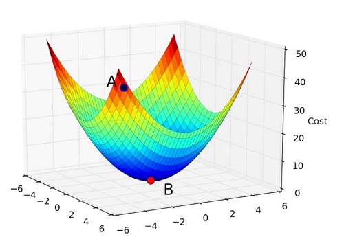
How terrifying the picture is as well as it’s formulas! But, it is actually not like how it looks. It is very easy, interesting and very practical concept.
So, let’s forget the terrifying plots, formulas and the bitter experiences and make a new start.
Some Basic Real-World Concept:
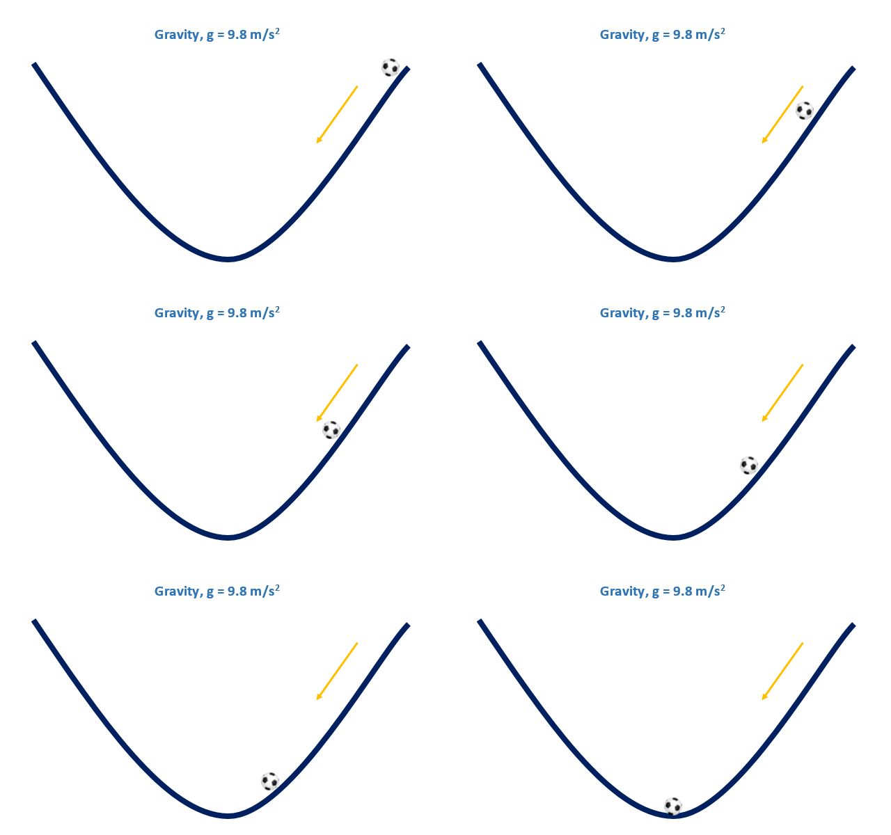
Let’s say, we put a ball on the upper edge of a pond and give a little push on it, just like the following picture. Now, what will happen?
Now, let’s discuss some childhood mathematical concepts.
Let, we have a function, $f(x) = x^2+5$, and we also have some values of $x$.
$x =−6,−5,−4,−3,−2,−1,0,1,2,3,4,5,6$
Now, our task is to find the minimum value of the function. That means, we need to find such an input value for the $x$ for which we’ll get the minimum output value from $y$.
Now, let’s put all the given values of $x$ into the function and see the output values of $y$.
| x | y = f(x) = x² + 5 |
|---|---|
| -6 | 41 |
| -5 | 30 |
| -4 | 21 |
| -3 | 14 |
| -2 | 9 |
| -1 | 6 |
| 0 | 5 |
| 1 | 6 |
| 2 | 9 |
| 3 | 14 |
| 4 | 21 |
| 5 | 30 |
| 6 | 41 |
From the table, we can see that when we put $0$ in $x$, we are getting the minimum value $5$ from $y$.
We can write the above function and generate it’s output in Python code as below –
import numpy as np

def func(x):
    return x**2+5

x = np.array([-6,-5,-4,-3,-2,-1,0,1,2,3,4,5,6])
y = func(x)

print(x)
print(y)
Output:
[-6 -5 -4 -3 -2 -1 0 1 2 3 4 5 6]
[41 30 21 14 9 6 5 6 9 14 21 30 41]
Now let’s see, for the given values how the function looks like in graphical representation.
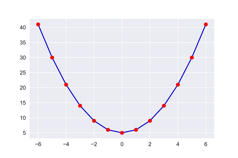
The most interesting fact here is, the plot looks same as the picture of the pond we’ve used above.
That’s great! Our learning has become much easier. 🤘
Now, if we put a ball on the upper edge of the plot and give a little push on it, as we done before in the pond picture. What will happen?
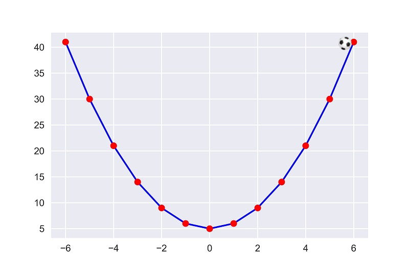
Nothing will happen. Because the gravitational force works on earth, not on our plot. The ball will remain in the same position where it was put before. Then, how can we take the ball to the minimum point of the graph?
To do this, we need to know 2 things-
- The direction of the slope (We can know this from the gradient.)
- By how many units we need to roll. (We can set this value by our own.)
Now, it’s time to know about the Gradient Descent. Let’s see how can it help us.
Gradient Descent:
Gradient Descent is a first order iterative optimization algorithm that finds the minimum value of a function.
We’ll know what it means by “first order” and “iterative” later.
The formula used in Gradient Descent:
$x_{n+1} = x_n - \gamma \cdot \nabla F(x_n)$
The formula will tell us the next position of the ball. It’ll tell us the direction of downward slope with the number of units to roll. You’ll find this formula written with different notation as follows–
- $\theta_1 = \theta_0 - \alpha \cdot f^{\prime}(\theta_0)$
- $a_{n+1} = a_n - \gamma \cdot \nabla F(a_n)$
Now, let’s learn the meaning of the notations used in the formula-
- $x_{n+1} =$ The new position. The direction of the downward slope with the number of units to roll.
- $x_n =$ The current position.
- $\gamma =$ Learning rate or step size. (We can set it by our own.)
- $\nabla F(x_n) =$ The gradient of function $F$ for the point $x_n$.
As we told before, we can set the value of $\gamma$ (Learning rate) and we can also set the current position of $x$. The thing we need to think about is how to find $\nabla F(x_n)$.
Finding the gradient of a function:
If we want to find the gradient of a function for a point $x$, we need to differentiate the function for once with respect to $x$.
The result we’ll get by differentiating the function once is called the first order derivative of that function.
So, let’s differentiate our function $f(x) = x^2 + 5$ and see what we get-
$x_{gradient} = \frac{d}{dx}\cdot f(x)$
$=> x_{gradient} = \frac{d}{dx} (x^2+5)$
$=> x_{gradient} = 2x$
If we’ve forgotten calculus, nothing to worry. The sympy package of Python can find the derivative of a function for us.
In the following python code, the sympy package will find the derivative for our function $f(x) = x^2 + 5$.
import sympy as sp

x = sp.Symbol('x')

f = x**2 + 5
f_prime = f.diff(x)

print(f_prime)
Output:
2*x
You can ask, why do we need to take the first derivate?
Reasons to take the first derivative:
- The first derivative tells us the direction of the function, whether the function is increasing or decreasing.
- The first derivative also tells us about the slope of the function.
Now, let’s understand why we call the gradient descent algorithm iterative. The formula for gradient descent we discussed above tells us the direction and number of units to roll for the next position. But we can’t reach the minimum point by rolling the ball once. We need to roll the ball for a certain number of times. We need to repeat the process until we achieve the convergence. That’s why we need to use a loop to repeat the process.
Let’s write the formula of the algorithm in a bit more nice way-
Repeat until convergence {
$x_{n+1} = x_n - \gamma \cdot \nabla F(x_n)$
}
Finally, we’ve known all the concepts that we need to write the code for gradient descent.
Let’s code the gradient descent quickly-
- We’ll set $0.001$ as the value of \gamma (gamma). If we set the value of learning rate larger, there is a chance to overtake the minimum point. That’s why we’ll take a good value for $γ$ which is $0.001$.
- Now, we need to set our starting point. That means we need to set an initial value for $x$, from where we’ll start rolling the ball. We’ll set the initial point $x = 6$.
- Finally, we need to set the number of iterations for the repeating process. We’ll set it to $5000$.
gamma = 0.001
x = 6
iterations = 5000

for i in range(0,iterations):
    x_gradient = 2*x
    x1 = x - gamma * x_gradient
    x = x1

print("iterations =",iterations,"\nx = ",x)
Output:
iterations = 5000
x = 0.00026968555624761565
Here we see that after $5000$ iterations we get a value of $0.00026968555624761565$ for $x$ which is very close to $0$. Actually, if we convert it to an integer, it’ll turn into $0$. So, we’ve got out expected minimum value $0$ for $x$ which will cause the function output the minimum value $5$.
Now if we look at the plot, we’ll see the ball is rolling down and reaches the minimum point of the plot.
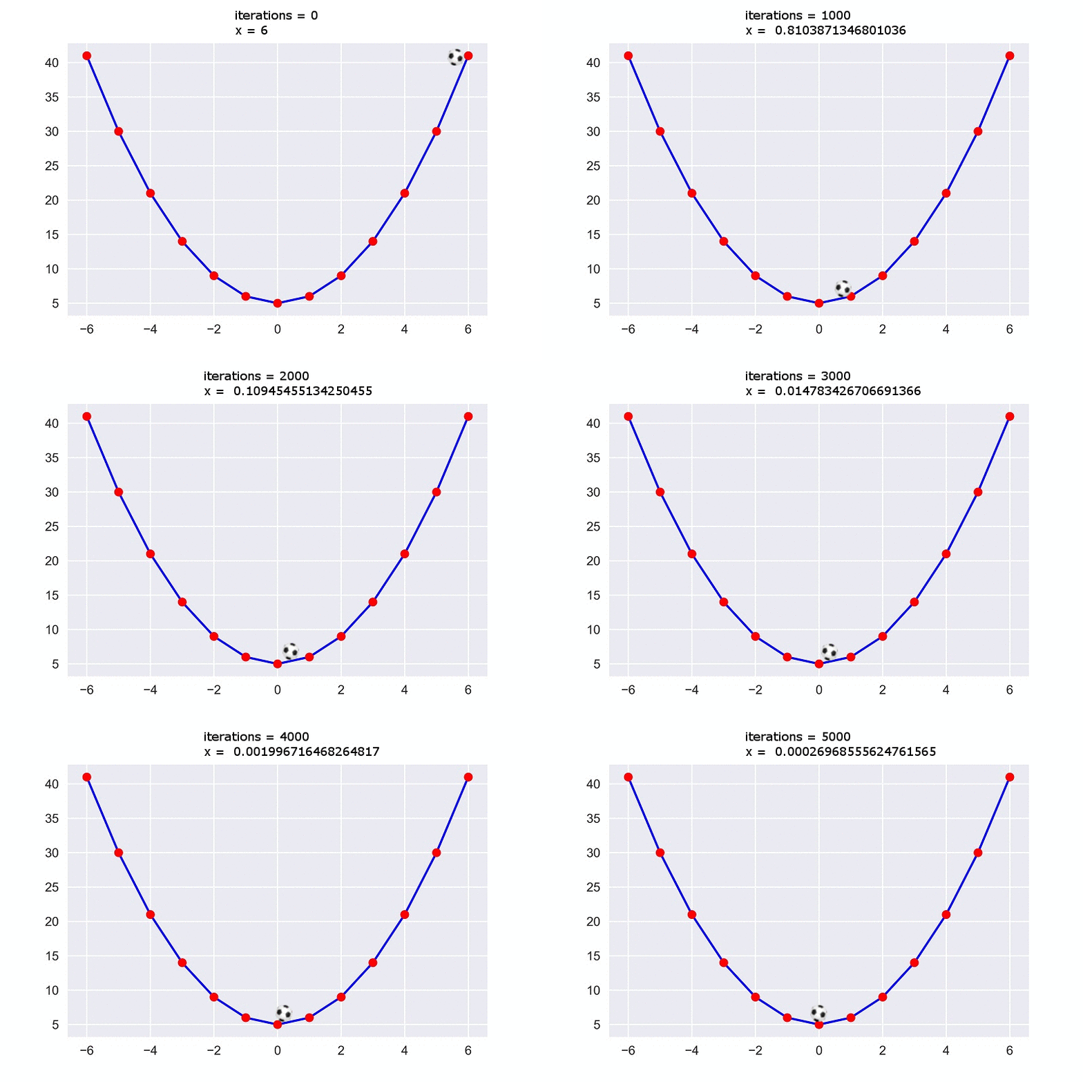
This is the intuition behind gradient descent algorithm.
In this article, I’ve used a simple function with one parameter. But to feel the real advantage of gradient descent, we need to work with multiple parameterized function. In the next article, I’ll show how can we use gradient descent to minimize the error of Linear Regression. There we’ll work with multiple parameters.
Till then practice what you’ve learnt from this article. ![]()
Constructive criticism will be appreciated.